Playing with a toy climate model

Happy Earth Day 2023! I’m redoing a post I did several years ago. This time, anyone who wants the code can get it from the post.

The premise is simple: Correlate global temperature with CO₂ levels, solar activity, El Niño/Southern Oscillation (ENSO), and aerosol levels via multiple regression, then use that regression model to retroactively predict changes in global temperatures from 1958 to present. This allows us to tease out the influence of different variables on global temperatures. Why 1958? That’s the first year we have continuious monthly atmospheric CO₂ data. So without further ado, here’s the model I created. First, let’s wrangle the data:

Show the code

library(tidyverse)
library(imputeTS)
library(Hmisc)

# Temperature data
GISS <- read_table("https://data.giss.nasa.gov/gistemp/tabledata_v4/GLB.Ts+dSST.txt",
                   skip = 7) %>%
        slice(1:(n() - 5)) %>%
        filter(!row_number() %in% c(22, 43, 64, 85, 106, 127, 148))
GISS[GISS == "****"] <- NA

GISS <- GISS %>% select("Year", 
                        "Jan", 
                        "Feb", 
                        "Mar", 
                        "Apr", 
                        "May", 
                        "Jun", 
                        "Jul", 
                        "Aug", 
                        "Sep", 
                        "Oct", 
                        "Nov", 
                        "Dec")

GISS$Year <- as.numeric(GISS$Year)
GISS$Jan <- as.numeric(GISS$Jan)
GISS$Feb <- as.numeric(GISS$Feb)
GISS$Mar <- as.numeric(GISS$Mar)
GISS$Apr <- as.numeric(GISS$Apr)
GISS$May <- as.numeric(GISS$May)
GISS$Jun <- as.numeric(GISS$Jun)
GISS$Jul <- as.numeric(GISS$Jul)
GISS$Aug <- as.numeric(GISS$Aug)
GISS$Sep <- as.numeric(GISS$Sep)
GISS$Oct <- as.numeric(GISS$Oct)
GISS$Nov <- as.numeric(GISS$Nov)
GISS$Dec <- as.numeric(GISS$Dec)

GISS <- GISS %>%
        pivot_longer(c(Jan, 
                       Feb, 
                       Mar, 
                       Apr,
                       May,
                       Jun,
                       Jul,
                       Aug,
                       Sep,
                       Oct,
                       Nov,
                       Dec), names_to = "Month", values_to = "anomaly") %>%
        mutate(time = dmy(paste(1, Month, Year))) %>%
        select(time, anomaly)
GISS$anomaly <- GISS$anomaly/100
GISS <- subset(GISS, time >= "1958-03-01") %>%
        rename(Temperature = anomaly)

# CO2 data
co2 <- read_table("https://gml.noaa.gov/webdata/ccgg/trends/co2/co2_mm_mlo.txt",
                  col_names = FALSE, skip = 58)

co2 <- co2 %>%
        select(X1, X2, X4) %>%
        rename(Year = X1, Month = X2, CO2 = X4) %>%
        mutate(time = make_date(year = Year, month = Month, day = 1 )) %>%
        mutate(CO2_rf = 5.35*log(CO2/280)) %>%
        select(time, CO2_rf) %>%
        rename(CO2 = CO2_rf)



# Sunspot data
sunspots <- read_table("https://www.sidc.be/silso/DATA/SN_m_tot_V2.0.txt",
                       col_names = FALSE)
sunspots <- sunspots %>%
        rename(Year = X1, Month = X2, sunspots = X4) %>%
        mutate(time = make_date(year = Year, month = Month, day = 1)) %>%
        select(time, sunspots) %>%
        subset(time >= "1957-12-01")
sunspots$sunspots_lagged <- Lag(sunspots$sunspots, 1) 
sunspots <- sunspots %>%
        subset(time >= "1958-03-01") %>%
        select(time, sunspots_lagged) %>%
        rename("Solar" = sunspots_lagged)

# ENSO data

ENSO <- read_table("https://www.cpc.ncep.noaa.gov/data/indices/oni.ascii.txt")
ENSO$time <- seq.Date(from = as.Date("1950-01-01"), by = "month", length.out = nrow(ENSO))
ENSO <- subset(ENSO, time >= "1957-09-01") %>%
        rename(ENSO = ANOM) %>%
        select(time, ENSO)
ENSO$ENSO_lagged <- Lag(ENSO$ENSO, 3)
ENSO <- ENSO %>%
        select(time, ENSO_lagged) %>%
        rename(ENSO = ENSO_lagged)

# Aerosols data

aerosols <- read_table("https://data.giss.nasa.gov/modelforce/strataer/tau.line_2012.12.txt",
                       skip = 3) %>%
        rename(time = "year/mon", Aerosols = global) %>%
        mutate_at(c("time", "Aerosols"), as.numeric) %>%
        select(time, Aerosols)

aerosols$time <- format(date_decimal(aerosols$time), "%Y-%m-01") %>%
        as.Date(aerosols$time, format = "%Y-%m-%d")
aerosols <- subset(aerosols, time >= "1955-10-01")

## Extrapolate out from 2012-09-01
length_out <- subset(ENSO, time >= "2012-10-01")
length_out <- length(length_out$time)

extrapolation <- data.frame(
        time = seq(from = as.Date("2012-10-01"), by = "1 month", length = length_out),
        Aerosols = "NaN"
)

aerosols <- rbind(aerosols, extrapolation)
aerosols$Aerosols <- as.numeric(aerosols$Aerosols)
aerosols <- na_interpolation(aerosols, option = "linear")
aerosols$Aerosols_lagged <- Lag(aerosols$Aerosols, 18)
aerosols <- aerosols %>%
        select(time, Aerosols_lagged) %>%
        rename(Aerosols = Aerosols_lagged)
aerosols <- subset(aerosols, time >= "1958-03-01")

# Make data frame

df_list <- list(GISS, co2, sunspots, ENSO, aerosols)
global_temp <- df_list %>%
        reduce(inner_join, by = "time") %>%
        mutate(date = decimal_date(time)) %>%
        select(date, Temperature, CO2, Solar, ENSO, Aerosols) %>%
        rename(time = date)

During the wrangling process, I converted CO₂ levels to radiative forcing using a formula from Myhre et al. (1998). I then lagged aerosols by 18 months, which lined up the El Chichon and Mount Pinatubo eruptions with their effect on global climate and used a linear extrapolation to extend the aerosol data set to 2023. Global temperatures lag changes in El Niño/Southern Oscillation by 3 months and solar activity by 1 month. I used multiple linear regression to create the model Temperatures ~ CO₂ + Solar + ENSO + Aerosols. Finally, I created a Shiny app that allows users to explore how predicted mean temperature change given any combination of those independent variables. You can find the app at https://jrmilks.shinyapps.io/Simple_Climate_model/.

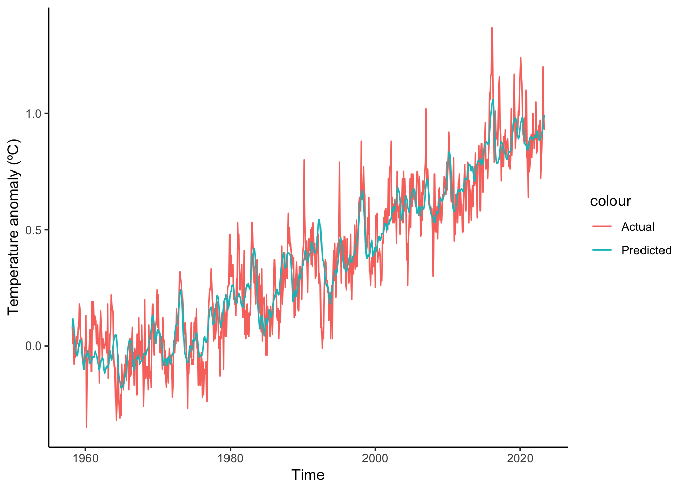
For those who want a preview, here’s the main model with all four variables in it:

Show the code

library(tidyverse)

Climate.fit <- lm(Temperature ~ CO2 + Solar + ENSO + Aerosols, data = global_temp)

trendFitData <- data.frame(time = global_temp$time, 
                           temperatureFit = Climate.fit$fitted.values)

p <- ggplot(data = global_temp, 
       aes(x = time,
           y = Temperature,
           colour = "Actual")) +
        theme_classic() +
        geom_line() +
        geom_line(data = trendFitData,
                  aes(x = time,
                      y = temperatureFit,
                      colour = "Predicted")) +
        labs(x = "Time",
             y = "Temperature anomaly (ºC)",
             main = "Actual vs predicted global mean temperature")
p

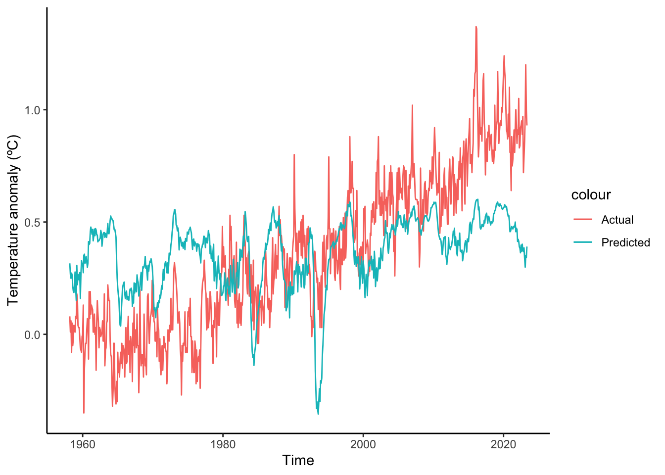
As you can see, the predicted global mean temperature matches the observed temperature fairly well, with R² = 0.8851. The observed trend is 1.67ºC per century. The predicted trend? 1.66ºC per century. Not too shabby of a fit. And here’s the fit without CO₂:

Show the code

library(tidyverse)

Climate.fit <- lm(Temperature ~ Solar + ENSO + Aerosols, data = global_temp)

trendFitData <- data.frame(time = global_temp$time, 
                           temperatureFit = Climate.fit$fitted.values)

p2 <- ggplot(data = global_temp, 
       aes(x = time,
           y = Temperature,
           colour = "Actual")) +
        theme_classic() +
        geom_line() +
        geom_line(data = trendFitData,
                  aes(x = time,
                      y = temperatureFit,
                      colour = "Predicted")) +
        labs(x = "Time",
             y = "Temperature anomaly (ºC)",
             main = "Actual vs predicted global mean temperature")

p2

Quite different and does not follow the observed trend at all. Actual mean temperature has been increasing by an average of 1.67ºC per century since 1958. Without CO₂, the predicted model trend is 0.32ºC per century since 1958. The combination of solar activity, ENSO, and aerosols matches the wriggles around the trend but cannot match the trend itself.

Anyway, take a look at the app. Want the code to the Shiny app? Go to https://jrmilks.shinyapps.io/Simple_Climate_model/. See anything wrong with my code or have suggested improvements? Drop me a line or leave a comment.

References

Myhre, Gunnar, Eleanor J. Highwood, Keith P. Shine, and Frode Stordal. 1998. “New Estimates of Radiative Forcing Due to Well Mixed Greenhouse Gases.” Geophysical Research Letters 25 (14): 2715–18. https://doi.org/10.1029/98gl01908.